📦 Session 1
Tensors: The powerhouse of a Neural Network
This first week we will explore what computer vision is and the fundamentals of Neural Networks.
Links:
🎥 Computer Vision?
Computer Vision is a field within artificial intelligence that focuses on enabling machines to interpret and understand visual information from the world, similar to how human vision operates. It originated in the 1970s with the ambition to replicate human sight, at institutes like MIT, Stanford and, CMU. The development of Computer Vision was initially slow, hampered by limited computing power and data. However, the advent of machine learning and, more significantly, deep learning technologies in the late 20th and early 21st centuries allowed for profound advancements. These included breakthroughs in image recognition, object detection, and semantic segmentation, leveraging large datasets and increased computational capabilities. Today, Computer Vision underpins a multitude of applications across various sectors, such as autonomous driving, security surveillance, healthcare, and augmented reality, demonstrating its critical role in the advancement of artificial intelligence and technology at large. Recently multimodality took the forefront, combining the power of Large Language Models such as ChatGPT 4 with vision capabilities.1
Computer Vision in the Humanities
Computer vision technologies have revolutionized the way we analyze visual and textual data in the Humanities. By automating the process of extracting information from images and documents, researchers can uncover insights at a scale previously unimaginable.
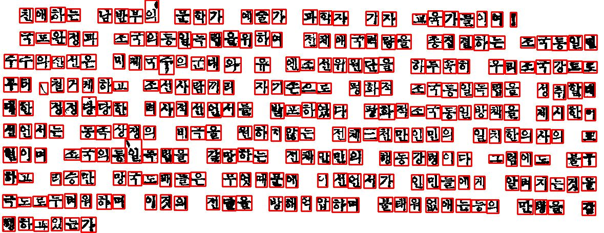


Examples of Computer Vision applications in the Humanities
Digitization and Preservation: OCR technology not only digitizes texts but also preserves historical documents, making them accessible for future generations. This process includes the transcription of manuscripts, letters, and books and more.
Artwork and Cultural Artifact Analysis: Computer Vision algorithms analyze visual patterns, colors, and shapes in artworks and artifacts, assisting in authenticity verification, restoration, and understanding artistic influences across different cultures and periods.
Pattern Recognition in Historical Data: By identifying patterns in archival materials, such as maps, photographs, and paintings, researchers can study changes in landscapes, urban development, and social movements over time.
Enhanced Manuscript Reading: Computer Vision aids in deciphering complex handwritten texts, including marginalia and annotations, providing deeper insights into the thought process3es and historical contexts of their authors.
Cultural Heritage Reconstructions: 3D modeling and reconstruction of archaeological sites and historical buildings allow researchers and the public to visualize and explore lost or damaged heritage sites.
Facial Recognition in Portraiture: This technology is used to study changes in portraiture styles, identify unknown subjects in historical paintings, and analyze cultural perceptions of beauty and identity across different eras.
For an in-depth exploration of computer vision’s impact on Humanities research, see: Wevers and Smits.2
🧠 Logic Networks and the Limits of Rule-Based Systems
Logic networks, or rule-based systems, represent knowledge in the form of logic patterns or conditional statements, typically expressed as \(A \rightarrow B\). For example, the statement “if it rains \((A)\), I am inside \((B)\)” illustrates a simple logic pattern where one condition directly leads to another. This approach is effective for clear-cut, straightforward rules but encounters significant limitations when addressing more complex or nuanced scenarios.
Consider the challenge of recognizing a cat 🐈 in an image. A logic-based approach might attempt to define a cat by a set of specific attributes:
- Whiskers?
- Tail?
- Ears?
However, the inherent complexity and variability of visual characteristics in different contexts make it exceedingly difficult to construct a comprehensive, rule-based system for accurate recognition. How do you account for the vast diversity of cat breeds, poses, sizes, or the ways a cat might partially be obscured in an image? The limitations of logic networks become apparent as the complexity of the question increases, highlighting the need for more advanced solutions to understand and interpret visual data effectively.
🧠 Neural Networks: Embracing Complexity through Learning
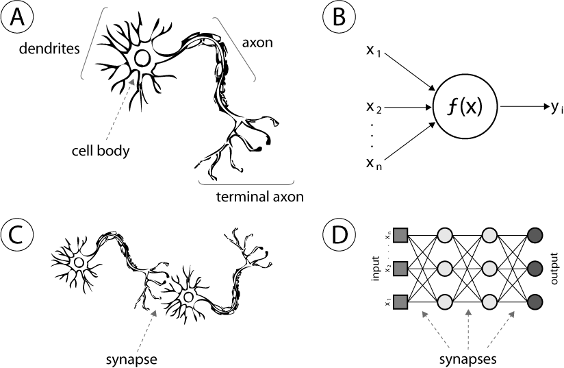
The strength of neural networks lies in their ability to adapt and learn from vast amounts of data, making them particularly effective for applications where the logic is too intricate or dynamic to be explicitly defined. Modeled after the human brain, these networks consist of interconnected nodes, or neurons, that process information collaboratively. They are able to accurately identifying the subtle features of animals in diverse images to parsing the complexities of human speech, neural networks have become a cornerstone of modern artificial intelligence.
Simply put, we provide the input and desired output, and let the Neural Network figure out the logic.
📦 Tensors: The Powerhouse of Neural Networks
Tensors are the core component that neural networks use to process information. Essentially, they are containers that can hold data in multiple dimensions, making them incredibly versatile for various types of input and output data, from simple numbers to complex images and beyond.
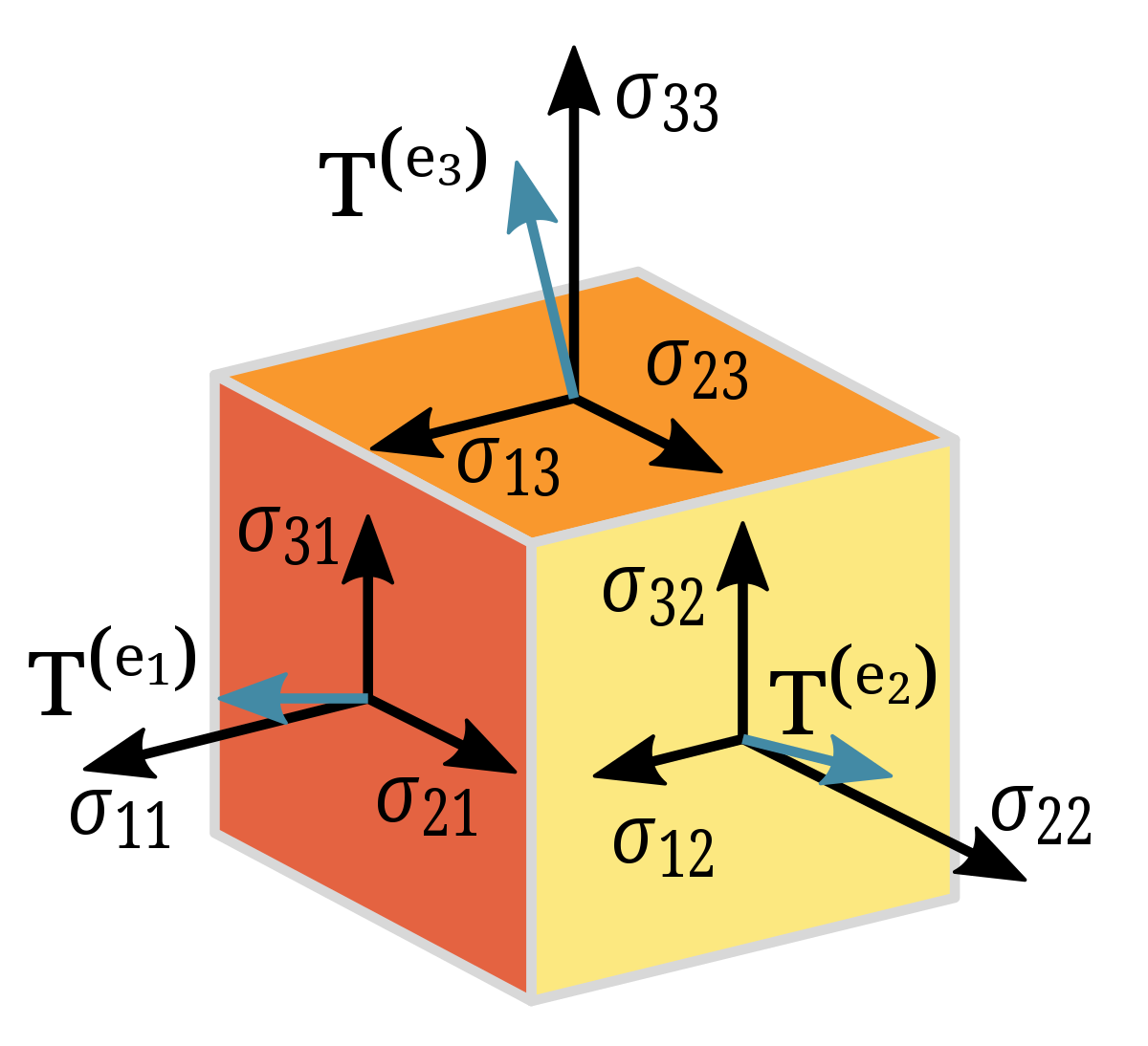
In the context of neural networks, tensors allow these systems to understand and manipulate the vast amounts of data they’re trained on, such as images, text, and sound. By organizing data into this multi-dimensional format, tensors allow neural networks to operate.
📦 What are Tensors?
Tensors are a fundamental concept in the field of machine learning and neural networks, acting as the main format for storing and processing data. To understand tensors better, let’s explore how they represent different types of data through examples.
From simple numerical data to complex images, tensors can encapsulate information in an organized, multi-dimensional structure. Below are examples illustrating how tensors represent various data forms, from scalar values to high-dimensional data like images.

In the image above, we can see the following representations.
- Scalar values (A single data point)
- Vectors (A list Data)
- Matrices (A list of Data Lists – each row being a list.)
- Cube Tensors (A list of lists of lists)
Each of the squares you see in this representation would hold a number that represents some kind of data. For example, image data. Images are often stored as pixel values on a computer. Each pixel that forms an image would hold a value. For grayscale images, each pixel is represented by a single value indicating its shade, ranging from black through various shades of gray to white. See the example of Lincoln below.
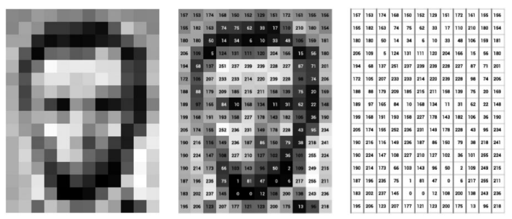
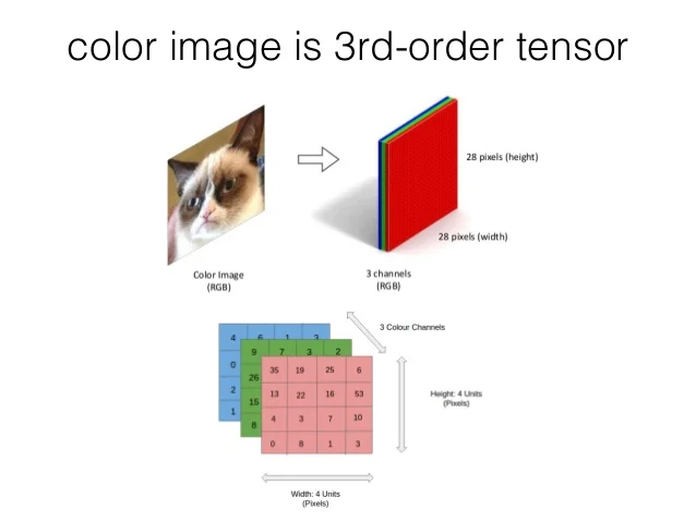
A grayscale image can thus be represented by a simple matrix (2D Tensor). However when we turn to colored images, this is not the case. Colored images consist of three color channels: Red, Green, and Blue (RGB). For an RGB image, a single pixel’s color is represented by a combination of three values, one for each color channel. Therefore, an RGB image is represented by three separate matrices where each matrix corresponds to one of the color channels. Which in this case would be a cube or more appropriately a 3D tensor. See the example below for a tensor of a colored image.
Tensors in code
A Scalar
A scalar represents a single value. In the context of tensors and PyTorch, even a simple number like 1 can be considered a tensor of zero dimension. Here’s how we conceptually represent a scalar:
# Scalar
1
A Vector
A vector is a 1-dimensional array of numbers, representing a sequence of scalar values. It can be thought of as a list of numbers arranged in a specific order. Here’s a simple example of a vector:
# Vector
[1,2,3]
A Matrix
A matrix extends the concept of a vector into two dimensions, consisting of rows and columns of numbers. It represents a collection of numbers arranged in a rectangular grid. Here’s an example of a 3x3 matrix:
# Matrix
[[1,2,3],
 [4,5,6],
 [7,8,9]]
A 3D Tensor (Cube)
A tensor can generalize scalars, vectors, and matrices to higher dimensions. A 3-dimensional tensor, for example, can be visualized as a cube of numbers, extending the matrix concept into the third dimension. Here’s how a simple 3D tensor, or a cube, can be represented:
 # Cube
[[[1,2,3],
  [4,5,6],
  [7,8,9]],
 [[1,2,3],
  [4,5,6],
  [7,8,9]]]
📏 Dimensions
Tensors are characterized by their dimensions, a fundamental property that describes their complexity and structure.
Tensors have a so-called dimension that is crucial for understanding their shape and the type of data they represent. A dimension can be thought of as how many numbers are required to locate a point within the tensor. For example, a scalar (a tensor of dimension 0) does not require any numbers to locate its point because it is a single point. A vector (a tensor of dimension 1) requires one number, a matrix (a tensor of dimension 2) requires two numbers, and so on.
It’s worth noting that the term degrees of freedom is often used interchangeably with dimension in the context of tensors. Essentially, both terms describe the number of independent ways in which the data within the tensor can vary.

- Scalar: 0 dimensions
- Characteristics: Represents a single value with no associated coordinates. Only one location is possible, the simplest form of a tensor.
- Vector: 1 dimension
- Characteristics: Requires one coordinate to specify a point within it. Think of it as a line where each point along the line is identified by a single number.
- Matrix: 2 dimensions
- Characteristics: Defined by two coordinates, like a flat surface. To locate a point, you need two numbers: one for the row and one for the column.
- Cube-Tensor (3D Tensor): 3 dimensions
- Characteristics: Requires three coordinates to locate a point, resembling a cube in space. This structure allows for the representation of more complex data, such as color images with dimensions for height, width, and color channels.
Sometimes you’ll encounter the term:
N-th Dimensional Tensor
The N refers to the number of dimensions of a tensor. This notation allows for the representation of tensors with any number of dimensions, accommodating a wide array of complex data structures beyond simple scalars, vectors, matrices, or even 3D tensors.
Example of a 4th Dimensional Tensor: An excellent example of a usable 4th dimensional tensor is colored video data. In this case, the dimensions represent:
- Height of the video frame
- Width of the video frame
- Color channels (RGB)
- The sequence of frames over time
This structure enables the tensor to capture not just the spatial layout of each frame in the video through its height, width, and color dimensions but also the temporal dimension through the sequence of frames.
Dimensions in Code
Counting the number of brackets at the start will tell you the number of dimensions.
# Scalar - 0 dimensions
# Represented by a simple value without any brackets.
1

# Vector - 1 dimension
# Represented by a list of values enclosed in a single set of brackets.
[1, 2, 3]

# Matrix - 2 dimensions
# Represented by a list of lists, with each inner list enclosed in its own set of brackets.
[[1, 2, 3],
 [4, 5, 6],
 [7, 8, 9]]

# Cube (3D Tensor) - 3 dimensions
# Represented by a list of matrices, with each matrix enclosed in its own set of brackets, nested within an outer list.
[[[1, 2, 3],
  [4, 5, 6],
  [7, 8, 9]],
 [[1, 2, 3],
  [4, 5, 6],
  [7, 8, 9]]]
📐 Shapes
Tensors are not just defined by their dimension but also by their shapes, an essential attribute that gives more detailed information about their structure.
Tensors have shapes that provide a precise way of describing their size and layout. The shape of a tensor refers to the number of elements it contains along each dimension.
This means that:
- A 1-D Tensor (or vector) has a shape represented as \((x)\), where \(x\) is the number of elements in the vector.
- A 2-D Tensor (or matrix) has a shape \((x, y)\), indicating \(x\) elements in rows and \(y\) elements in columns.
- A 3-D Tensor has a shape \((x, y, z)\), denoting \(x\) elements in the first dimension (e.g., depth), \(y\) elements in the second dimension (e.g., rows), and \(z\) elements in the third dimension (e.g., columns).
- And so on for higher-dimensional tensors…
Take this representation of a single 3D Tensor

[[[ 0,  1,  2,  3,  4],
  [ 5,  6,  7,  8,  9]],

 [[10, 11, 12, 13, 14],
  [15, 16, 17, 18, 19]],

 [[20, 21, 22, 23, 24],
  [25, 26, 27, 28, 29]]]
Working from outer bracket to inner bracket, this 3D tensor consists of three 2D matrices, each with 2 rows and 5 columns, illustrating how data can be organized in multiple dimensions within a tensor. Hence its shape is (3,2,5).
🙋 Why learn this?
Most issues you will encounter in while working with Neural Networks are shape errors.
RuntimeError: mat1 and mat2 shapes cannot be multiplied (3x4 and 3x4)
- Without knowing dimensions and shapes, you can not solve errors like this.
- Often as researchers we only care about the dimension and shapes of Tensors.
🔥 PyTorch
In our exploration of computer vision for the humanities, we will utilize PyTorch, a powerful and flexible open-source machine learning library. By leveraging PyTorch, we can easily manipulate tensors, perform automatic differentiation, and accelerate computations using GPU acceleration, enabling the efficient development and training of models.8
You can import PyTorch in Python:
import torchTensors in Pytorch
Here’s a brief explanation of some foundational operations and attributes related to tensors in PyTorch:
torch.tensor()
The torch.tensor function is used to create a tensor in PyTorch. This function allows you to directly convert data into a tensor, including lists, arrays, and other numerical values. It’s the most straightforward way to create tensors for further manipulation and computation.
x = torch.tensor([1, 2, 3, 4])torch.rand()
torch.rand generates a tensor of a specified shape with random numbers drawn from a uniform distribution between 0 and 1. It’s particularly useful for initializing weights in neural networks or generating random data for testing. We input the shape we want as argument.
y = torch.rand(2, 3)  # Creates a 2x3 tensor with random values
z = torch.rand(5, 7)  # Creates a 5x7 tensor with random values
tensor.ndim
tensor.ndim is an attribute that returns the number of dimensions of a tensor (also known as its rank). You need the print() statement to show the output outside of a juypter cell.
x = torch.tensor([1, 2, 3, 4])
print(x.ndim)  # Outputs the number of dimensions in tensor x
tensor.shape
tensor.shape is an attribute that provides the shape of a tensor, represented as a tuple of its dimensions. Knowing the shape is essential for many tensor operations, including reshaping, slicing, and splitting tensors.
y = torch.rand(2, 3)
print(y.shape)  # Outputs the shape of tensor y
torch.arange()
torch.arange() creates a 1D tensor containing a sequence of numbers that range from a start value to an end value with a specified step size. It’s similar to the range function in Python and is useful for generating sequences of numbers. As arguments you usually set the start, end, and step. For decreasing numbers you would use a negative step.
z = torch.arange(start=0, end=5, step=1) # Creates a tensor [0, 1, 2, 3, 4]💿 Tensor Datatypes
In PyTorch, tensors can be of various datatypes, similar to standard Python integers, floats, or elements of Numpy arrays. The datatype of a tensor determines how much space it occupies in memory and how the bits are interpreted for mathematical operations.
torch.float32or simplytorch.float: Standard floating-point type; used for most computations and storage of neural network weights. It offers a good balance between precision and performance.torch.float16ortorch.half: Half precision floating-point type; uses half as many bits asfloat32. This datatype is particularly useful for reducing memory and computational requirements, especially on supported GPUs, while still providing sufficient precision for many deep learning tasks.
For more on PyTorch datatypes. See the documentation.
X = torch.rand(1,2)
print(X.dtype)
> torch.float32
🖥️ Tensor Devices
In PyTorch, tensors are not only defined by their shape and datatype but also by the device on which they reside. The device attribute of a tensor specifies whether it’s located on the CPU, a GPU, or other types of computing devices. Utilizing different devices can significantly impact the performance of your computations, especially for parallel processing tasks common in deep learning.
Common Devices
cpu: Utilizes the central processing unit of a computer. Suitable for tasks that don’t require heavy parallel computation.cuda: Refers to the use of NVIDIA GPUs, enabling accelerated computation by leveraging thousands of small, efficient cores suited for parallel tasks.mps: Represents GPU devices on Mac computers, utilizing Metal Performance Shaders for acceleration.tpu: Short for Tensor Processing Units, these are specialized hardware developed by Google for accelerating tensor computations.
Checking and Setting a Tensor’s Device
To check the current device of a tensor, use the .device attribute. By default, tensors are created on the CPU:
X = torch.rand(1,2)
print(X.device)
> device(type='cpu')
To move tensors between devices, you can use the .to() method. This is essential for leveraging GPU acceleration:
X = torch.rand(1,2).to('cuda')
print(X.device)
> device(type='cuda:0')
The 0 in cuda:0 refers to which GPU the tensor is on. Sometimes you have multipe GPUs and the second one would be cuda:1.
Note that moving tensors to a GPU is only possible if CUDA is supported and available on your system.
In Google Collab we need to activate the CUDA device by going to the menu item runtime > change runtime type > T4 GPU
❌ Datatype & Device Errors
Besides shape errors, the two other most common issues you’ll encounter are related to tensor datatypes (dtype) and the devices (device) on which tensors are stored.
Datatype Errors (dtype errors): These occur when you perform operations on tensors of incompatible datatypes, such as trying to add or multiply tensors of different precision levels (e.g.,torch.float32withtorch.float16).Device Errors (device errors): These happen when you attempt to perform tensor operations across tensors located on different devices, like trying to add a tensor on the CPU (device='cpu') with one on the GPU (device='cuda').
🧮 Tensor Operations
Tensor operations are the core mechanisms through which deep learning models learn, adapt, and make predictions. These operations can range from simple calculations to matrix multiplications.
🧮 Simple Operations
Addition
Adding a scalar value to a tensor increments each element of the tensor by that value. Similarly, adding two tensors together combines them element-wise.
# Adding a scalar
[1,2,3] + 2       = [3,4,5]

# Adding two tensors
[1,2,3] + [3,2,1] = [4,4,4]
Subtraction
Subtraction works similarly to addition, where a scalar value is subtracted from each element of the tensor, or two tensors are subtracted element-wise.
# Subtracting a scalar
[1,2,3] - 2       = [-1,0,1]

# Subtracting two tensors
[1,2,3] - [3,2,3] = [-2,0,0]
Multiplication (element-wise)
Element-wise multiplication can be performed between a tensor and a scalar or between two tensors. This operation multiplies each element by the scalar or corresponding element from the other tensor.
# Multiplying by a scalar
[1,2,3] * 2       = [2,4,6]

# Element-wise multiplication of two tensors
[1,2,3] * [3,2,3] = [3,4,9]
Division
Division operations are applied element-wise for both scalar division and division between two tensors.
# Dividing by a scalar
[1,2,3] / 2       = [0.5000,1.0000,1.5000]

# Element-wise division of two tensors
[1,2,3] / [3,2,3] = [0.3333,1.0000,1.0000]
🧮 Matrix Multiplication
Matrix multiplication sits at the heart of neural network operations, enabling the complex transformations and learning capabilities that define these models. While the actual computation of matrix multiplication is handled efficiently by libraries like PyTorch, understanding its principles is essential for anyone working with deep learning.
- MatMul efficiency is one of the most substantial computational bottlenecks.
- Matrix multiplication is often referred to as MM or MatMuls
Basic Rules
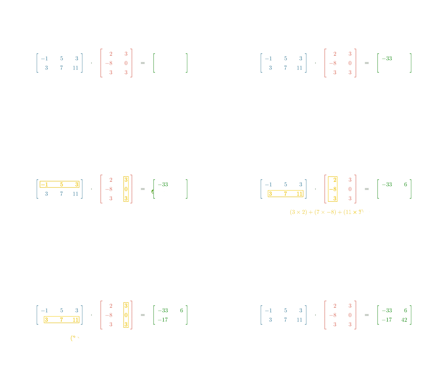
When multiplying two tensors, such as a tensor with shape (2x3) by a tensor with shape (3x2), there are a couple of fundamental rules to follow:
- Inner Dimensions Must Match: The inner dimensions of the matrices being multiplied must match. For example, in a multiplication (2x3) * (3x2), the inner dimensions are both 3, allowing the operation to proceed.
- Resulting Shape: The shape of the resulting tensor is determined by the outer dimensions of the matrices involved. Thus, when multiplying a (2x3) by a (3x2) matrix, the resulting tensor will have the shape (2x2), reflecting the outer dimensions.

To calculate the product (Matrix C):
- Element c1: Multiply each element of the first row of Matrix A by the corresponding element of the first column of Matrix B, then sum these products.
- Element c2: Multiply each element of the first row of Matrix A by the corresponding element of the second column of Matrix B, then sum these products.
- Element c3: Multiply each element of the second row of Matrix A by the corresponding element of the first column of Matrix B, then sum these products.
- Element c4: Multiply each element of the second row of Matrix A by the corresponding element of the second column of Matrix B, then sum these products.
The calculations for the elements of Matrix C are as follows:
- \(c1 = (a1 * b1) + (a2 * b3) + (a3 * b5)\)
- \(c2 = (a1 * b2) + (a2 * b4) + (a3 * b6)\)
- \(c3 = (a4 * b1) + (a5 * b3) + (a6 * b5)\)
- \(c4 = (a4 * b2) + (a5 * b4) + (a6 * b6)\)
These elements make up the resulting Matrix C after the multiplication.
Made with Manim
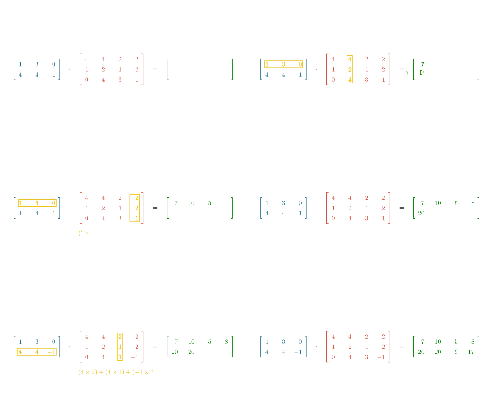
another way to visualise how Matrix Multiplication works is by checking out the following website and testing a few examples.
🛠️ Reshaping Tensors
Reshaping tensors is an essential technique in PyTorch that facilitates the reconfiguration of tensor dimensions without changing the underlying data. It is particularly useful in preparing tensors for different neural network layers that may require specific input shapes. The process includes several key operations:
🔧 Transposing
Transposing is an operation in tensor manipulation that flips the dimensions of a matrix or higher-dimensional tensor. This operation swaps the rows and columns of a 2D tensor, and in higher dimensions, it can swap two specified dimensions.
Why Transpose?
- Matrix Multiplication Compatibility: Transposing is particularly useful when you want to multiply two tensors that do not align dimensionally. For matrix multiplication to be valid, the number of columns in the first matrix must match the number of rows in the second matrix. Transposing adjusts the shape to meet this requirement.
- Data Reformatting: Sometimes data is loaded or generated in a format that isn’t suitable for the required operations, and transposing allows you to reformat it correctly.
Transposing in PyTorch
In PyTorch, you can transpose a tensor using the .T attribute for 2D tensors. For tensors with more than two dimensions, you would typically use the torch.transpose() function, specifying the dimensions you want to swap.
Here’s an example of transposing a 2D tensor from shape (4, 8) to (8, 4):
X = torch.rand(4, 8)       # Create a random tensor of shape (4, 8)
X_transposed = X.T         # Transpose the tensor
print(X_transposed.shape)  # Check the new shape of the tensor
# Output: torch.Size([8, 4])
🪚 Squeezing
Squeezing is an operation in tensor manipulation that involves removing singleton dimensions, or dimensions with a size of one. This process helps streamline the shape of a tensor for certain operations where dimensions of size one are not necessary.

It might look like the squeeze() operation would yield different results on these tensors depending on which of the dimensions remove. But whichever part you choose, you will always end up with the same 2D Tensor.
How Squeezing Works in PyTorch
In PyTorch, squeezing a tensor is performed using the .squeeze() method. This method finds all dimensions with a size of one and removes them, effectively “squeezing” the tensor down to fewer dimensions.
For example, a tensor with the shape (2, 1, 2) would become (2, 2) after squeezing. Visually, you can imagine this as removing unnecessary brackets from the tensor representation.
Here’s an example of applying the .squeeze() method:
X = torch.rand((2, 1, 2))  # Create a tensor with a singleton dimension
X_squeezed = X.squeeze()   # Squeeze the tensor to remove dimensions of size one
print(X_squeezed.shape)    # Output the new shape of the tensor
# Output: torch.Size([2, 2])
🔨 Unsqueezing
Unsqueezing is a tensor operation that adds a dimension with a size of one to a tensor at a specified position, essentially the inverse of squeezing. It’s a crucial operation when you need to adjust the dimensions of a tensor for certain PyTorch functions that expect inputs with a specific number of dimensions.
When you unsqueeze a tensor, you are not changing the data within the tensor but simply adding a new dimension that expands the shape of the tensor. This operation is important for aligning tensor shapes for operations like concatenation or when an operation requires a specific input dimensionality.

For instance, a tensor with the shape (2, 2) can be reshaped to:
(1, 2, 2)by unsqueezing atdim=0.(2, 1, 2)by unsqueezing atdim=1.(2, 2, 1)by unsqueezing atdim=2.
dim=3 would not work on a tensor with shape (2,2) as there is not yet ‘3rd’ index to add it. You will get a IndexError: Dimension out of Range.
Unsqueezing in PyTorch
In PyTorch, unsqueezing is done using the .unsqueeze(dim) method, where dim is the index at which the new dimension will be inserted.
X = torch.rand(2, 2)    # Create a tensor of shape (2, 2)
X_unsqueezed = X.unsqueeze(0)  # Add a new dimension at dim=0
print(X_unsqueezed.shape)     # Output the new shape of the tensor
# Output: torch.Size([1, 2, 2])
📈 Next Session: Linear Regression
