🎞️ Session 4
Images as Data
This session will revolve around images as data. The main focuses here will be:
- Loading images into tensors
- Batching & Dataloaders
- Creating model architectures for image data.
🎞️ Images as data
In the previous session, we have worked on generated datasets. These are excellent to learn the fundamentals of machine learning and deep learning. For many of us in the humanities, however, we rarely work with data that already in the form of numbers. Most of the time we work on textual data. If anything the digital humanities is a text focused field.
We see this throughout the field. Gold and Klein1 defined DH as follows:
Digital archives, quantitative analysis, and tool building projects.
Or a definition of DH by Oxford:
Text based and desk based
Most of the texts that are digitally accessible, are often not machine readable. Changing a text into machine readable form through OCR (Optical Character Recognition) takes significant effort. This means that most of the texts in archives are accessible as images, often JPG or PNG files. At the same time, a lot of fields in the humanities don’t only deal with texts as their main source. Take art history or any other subfield concerning itself with visual materials. Simply put, the humanities has a lot of potential for digitally processing images. This is exactly what neural networks have excelled in when compared to the more traditional approaches.
Thinking back to session 1, this is because it is hard to describe the exact rules needed to categorize visual materials. How do you differentiate a cat from a dog?
FashionMNIST
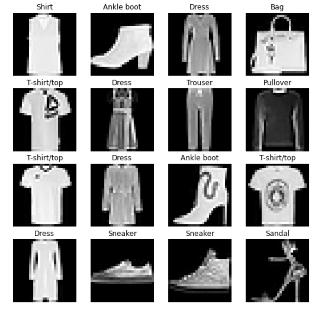
For this session, we will work with one of the most commonly used practice datasets available, the FashionMNIST dataset. This dataset was produced from images taken from Zalando products. It contains 70,000 gray-scale images in a 28*28px format with 9 classes.
- T-shirt/top
- Trouser
- Pullover
- Dress
- Coat
- Sandal
- Shirt
- Sneaker
- Bag
- Ankle boot

With this dataset, we thus aim to predict what class an image belongs to.
X data = Width*Height pixels of the image y data = Label (0-9) representing the class
PyTorch has already loaded in the images for us in the torch.datasets.FashionMNIST() so we do not need to load in the images ourselves. We will do this in the upcoming sessions.
However, we run into one issue that we haven’t faced before - the size of the data. 1000 data points can be pushed into the model all at once, but with larger datasets, it is more computationally efficient to batch the data.
📚 Batching and Dataloaders
As mentioned, batching allows us to work on large datasets and still be efficient with our computing power. We split the dataset into batches of N and feed those into our model. Let’s dive a bit more into some terminology.
Sample A sample is the smallest unit here, this represents a single data point, or in our case, a single image.
Batch size This is the hyperparameter that defines the number of samples per batch before updating the models’ parameters.
Epoch One full pass over the data, in case of batching, this means that one epoch is reached after all training batches have gone through the model.
Batch sizes are commonly chosen to be a power of two. 2 > 4 > 8 > 16 >32 etc etc.
What happens if the dataset doesn’t divide evenly by the batch size? The last batch simply gets less samples in it.
Batching in PyTorch has been made very simple by the introduction of dataloaders. These efficiently load in the data for us and also allow for a batch size parameter to be set.
We usually create two dataloaders the train_dataloader containing the samples for training, and the test_dataloader containing the samples for testing.
from torch.utils.data import DataLoader

# Setup the batch size hyperparameter
BATCH_SIZE = 32

# Turn datasets into iterables (batches)
train_dataloader = DataLoader(train_data, # dataset to turn into iterable
    batch_size=BATCH_SIZE, # how many samples per batch?
    shuffle=True # shuffle data every epoch?
)

test_dataloader = DataLoader(test_data,
    batch_size=BATCH_SIZE,
    shuffle=False # don't necessarily have to shuffle the testing data
)
The Dataloader can take in quite a few arguments, but for us the most important one besides the data and batch size is the shuffle parameter. For training we do want to shuffle as we don’t want the model to remember any kind of order. For our test set this doesn’t matter as we are not updating parameters when running it.
With this out of the way, we can work towards a baseline model.
🔧 Model Architectures for image data
🏗️ Baseline model
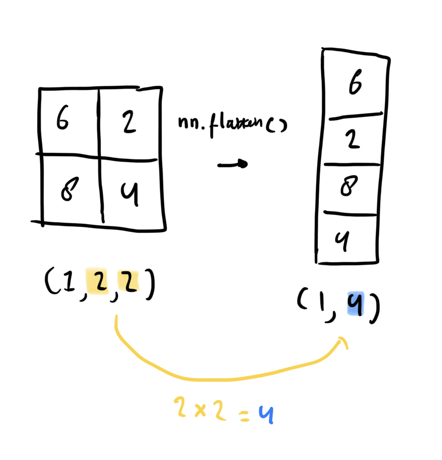
Unlike previous models, we’re working with image data, if we want to use `nn.Linear() layers with this data, we need to flatten it. This is done with nn.Flatten().
Visually this is easiest to explain:

# Create a flatten layer
flatten_model = nn.Flatten() # all nn modules function as a model (can do a forward pass)

# Get a single sample
x = train_features_batch[0]

# Flatten the sample
output = flatten_model(x) # perform forward pass

# Print out what happened
print(f"Shape before flattening: {x.shape} -> [color_channels, height, width]")
print(f"Shape after flattening: {output.shape} -> [color_channels, height*width]")

#returns
Shape before flattening: torch.Size([1, 28, 28]) -> [color_channels, height, width]
Shape after flattening: torch.Size([1, 784]) -> [color_channels, height*width]
With this transformation, linear layers can accept our image data.
Let’s construct a simple model:
# Create a model with non-linear and linear layers
class FashionModelV0(nn.Module):
    def __init__(self):
        super().__init__()
        self.layer_stack = nn.Sequential(
            nn.Flatten(), # flatten inputs into single vector
            nn.Linear(in_features=784, out_features=10),
            nn.ReLU(),
            nn.Linear(in_features=10, out_features=len(class_names)),
            nn.ReLU()
        )

    def forward(self, x: torch.Tensor):
        return self.layer_stack(x)
Training/Test Loop with batching
The train/test loop now also changes slightly as we have to loop over the batches as well as epochs.
The loss we calculate here is per batch, but we cant to update per epoch, which means we have to track the loss and calculate the average if we want to display it properly
epochs = 10

for epoch in range(epochs): # loop over epochs
    print(f'epoch:{epoch}')
    train_loss = 0 # tracking the loss
    for batch, (X, y) in enumrate(train_dataloader): # loop over batches
        X, y = X.to(device), y.to(device) # push batch to GPU
        model_1.train()

        # 1. Forward pass
        y_pred = model_1(X)
        loss = loss_fn(y_pred, y)
        train_loss += loss # accumulatively add up the loss per epoch

        # rest of the training loop...


    # Divide total train loss by length of train dataloader (average loss per batch per epoch)
    train_loss /= len(train_dataloader)

    # rest of the test loop...
After running this for 10 epochs, you’ll see decent performance, but nothing that would make this question a ‘solved issue’. If we want to improve our model further, we need to move beyond linear layers in combination with activation functions.
🧮 Convolutional Layers
Convolutional Neural Networks (CNN or ConvNet) are known for their ability to find patterns in visual data. The name comes from the mathematical concept of a convolution. A convolution is defined as:
‘an integral that expresses the amount of overlap of one function g as it is shifted over another function f’2
I will skip over much of the interesting mathematics behind this concept in favor of demonstrating its practical applications in our case, but I highly recommend you to watch this video from 3Blue1Brown which does an excellent job of explaining the intuition behind a convolution and how it is applied in practice too. If at any moment you are having trouble following what a convolution is, please give this video a chance.
Convolutions are widely used in image processing. For example, if you want to blur an image, you are essentially applying a convolution, if you are sharpening an image, you are applying a convolution, and so on…
Let’s go over a single convolution on an image.
- We have our image (in case of the definition function f)
- We have a kernel that applies some calculation to the pixels it ‘slides’ over. In this case the kernel is 33. (this is function g*)
- The result of the calculation is a single pixel value for a ‘new’ image.
- Slide over all the pixels to get a ‘compressed’ image.
Animation using manim taken from: https://github.com/i13abe/ConvAnimation/tree/main
In this animation, the numbers inside the kernel are static, but in our neural network, it is this kernel that constantly gets updated weights and biases to improve the performance of our model.
I’ll discuss the CNN-explainer website in more detail during the life session, but the text on the website also explains convolutions in a CNN very well.
We will copy the TinyVGG architecture you’ve seen on the CNN-explainer.
In TinyVGG a layer block has the following steps:
- 1st Conv2d layer (the convolution layer)
- ReLU activation function
- 2nd Conv2d layer
- ReLU activation function
- MaxPool2d layer (compressing the image even further)
This is repeated over two times, after which the classification layer comes.
We can write this out as follows in PyTorch
# Create a convolutional neural network
class FashionModelV1(nn.Module):
    """
    Model architecture copying TinyVGG
    """
    def __init__(self):
        super().__init__()
        self.block_1 = nn.Sequential(
            nn.Conv2d(in_channels=1,
                      out_channels=10,
                      kernel_size=3, # how big is the square that's going over the image?
                      stride=1, # default
                      padding=1),# options = "valid" (no padding) or "same" (output has same shape as input) or int for specific number
            nn.ReLU(),
            nn.Conv2d(in_channels=10,
                      out_channels=10,
                      kernel_size=3,
                      stride=1,
                      padding=1),
            nn.ReLU(),
            nn.MaxPool2d(kernel_size=2,
                         stride=2) # default stride value is same as kernel_size
        )
        self.block_2 = nn.Sequential(
            nn.Conv2d(10, 10, 3, padding=1),
            nn.ReLU(),
            nn.Conv2d(10, 10, 3, padding=1),
            nn.ReLU(),
            nn.MaxPool2d(2)
        )
        self.classifier = nn.Sequential(
            nn.Flatten(),
            # Where did this in_features shape come from?
            # It's because each layer of our network compresses and changes the shape of our inputs data.
            nn.Linear(in_features=10*7*7,
                      out_features=len(class_names))
        )

    def forward(self, x: torch.Tensor):
        x = self.block_1(x)
        # print(x.shape)
        x = self.block_2(x)
        # print(x.shape)
        x = self.classifier(x)
        # print(x.shape)
        return x
With this model, you’ll see that within 10 epochs you can get around 90% or higher on the accuracy score. With a little more you’ll achieve very good performance when compared to the base model that includes only linear layers and activation functions.
Confusion matrix
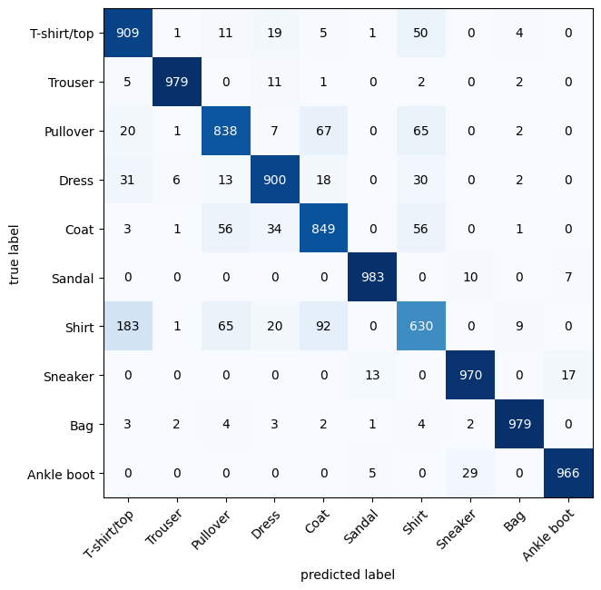
Let’s look at the confusion matrix for our model to examine its performance. We can do this with a new library called torchmetrics & mlxtend

As you can see the model performs quite well! I had reached 90% accuracy within 10 epochs. When examining this dataset, is the problem that the model still has a ‘model’ problem. That being, should we adjust the architecture further? Or when you take the confusion matrix into account, is it a ‘label’ problem?
A team at the company cleanlab examined FashionMNIST and found some interesting results… https://cleanlab.ai/blog/csa/csa-4/
📅 Next Session
Custom data & Transfer Learning
