⭕️ Session 3

Non-linear data with Neural Networks

This session will mainly focus on adjusting the architecture of our network to fit data beyond linearity. This is important as the layer types in this session will be part of the basic building blocks for our computer vision networks.

• 📑 Slides
• 🧑‍💻 Code
• ✅ Answers

⭕️ Non linearity

Last session we focused on linear data, fitting a linear line (regression) to data points. While surely a problem that occurs commonly in both research and industry, not all data can be neatly described by a linear function. Often we find this in so-called classification problems. It is exactly here that Neural Networks have set themselves apart from other types of machine learning. We can fit them to hard-to-describe data.

So what is a classification problem? It is in essence predicting whether something is one, or one of other classes. Within this we can make the following distinctions:

Problem type	What is it?	Example
Binary classification	Target can be one of two options, e.g. yes or no	Predict whether someone has heart disease based on their health parameters.
Multi-class classification	Target can be one of more than two options	Decide whether a photo of is of pizza, a hamburger or an ice cream.
Multi-label classification	Target can be assigned more than one option	Predict what categories should be assigned to a Wikipedia article (e.g. mathematics, science & philosophy).

A few examples of such data:

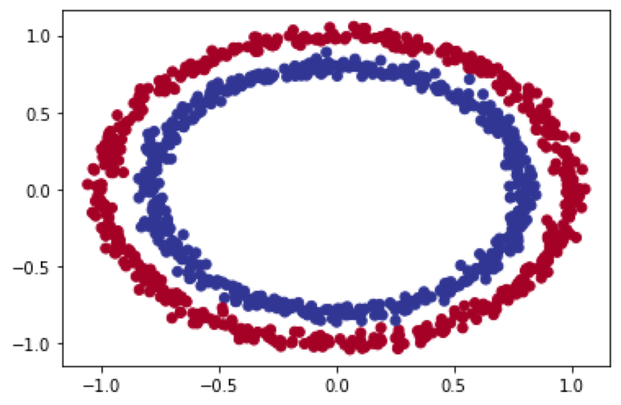
(a) make_circles() dataset

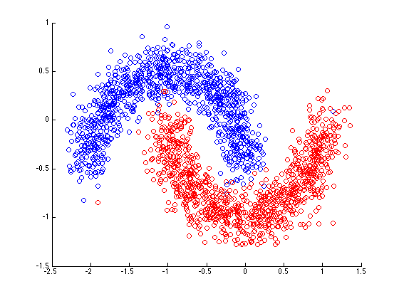
(b) make_moons() dataset

Figure 1: Examples of Non-linear datasets.

Both datasets can be generated using the sklearn.datasets make_circles() & make_moons(). See the documentation

To fit a model to such data, the model needs to be able to ‘bend’ its decision boundaries.

Creating Non-linear data

In order to create a Non-linear dataset we will again use the sklearn package as visualized above. This is an ideal library for generated some toy datasets. We will make use of the make_circles() function for the first generation.

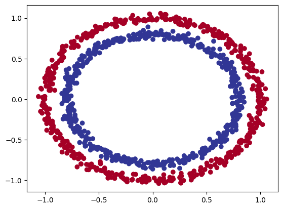
Figure 2: The generated make_circles() data

To generate this we use the following code:

# Make 1000 samples 
n_samples = 1000

# Create circles
X, y = make_circles(n_samples,
                    noise=0.03, # a bit of noise to the dots
                    random_state=448) # keep random state, so we get the same values

This returns us two numpy arrays. X holds the horizontal and vertical positions of the data points (x & y). y holds the numerical label for the corresponding data points.

However, we need to transform these still to torch.tensor format.

X = torch.from_numpy(X).type(torch.float)
y = torch.from_numpy(y).type(torch.float)

After this we again need to split our dataset. Remember to use sklearn for this!

# Split data into train and test sets
X_train, X_test, y_train, y_test = train_test_split(X, y, test_size=0.2) # 20% test, 80% train 

len(X_train), len(X_test), len(y_train), len(y_test)

With this dataset we can experiment on how to introduce non-linearity into a model.

🏗️ Model Construction - Base model

To demonstrate how architecture can influence the model, creating a base linear model to adjust later can demonstrate this well.

from torch import nn

class NL_ModelV0(nn.Module):
    def __init__(self):
        super().__init__()
        # Create nn.Linear layers capable of handling X and y input and output shapes
        self.network = nn.Sequential(
            nn.Linear(in_features=2, out_features=10), # takes in 2 features (X), produces 5 features
            nn.Linear(in_features=10, out_features=10), # 10 > 10
            nn.Linear(in_features=10, out_features=1), # 10 > 1
            )
    
    # Define a forward method containing the forward pass computation
    def forward(self, x):
        return self.network(x)

If we visualize this network we get the following:

Figure 3: A visualization of the produced network.

Image generated with the wonderful visualizer by Alexander Lenail

There are a few things to note on the correspondence of our code and the visualization:

• The starting data points match the in_features of our first nn.linear() layer.
• The two hidden layers match the first layers’ out_features and the second layers in_features.
• The final out_features matches the amount of classes we want to predict. Since we are working in a binary classification, we need only one neuron if it doesn’t activate (0) it is that class, if it does, it is the other (1).

🦾 Training for Classification

🔢 Logits

Before we continue into training, we must be aware of the differences between a predicted class, prediction probability and the raw model output. The latter is commonly referred to as the models logits. Logits are hard to keep track of as they hold no clear external meaning and can obscure a models’ confidence. This is why we normalize these values so the output of a models output layer sums to 1. How we do this differs if we are doing a binary or multi-class classification. In our case, we are working on a binary problem. Thus, we can use the torch.sigmoid() function.

If you want to learn more about the torch.sigmoid() function, please see the documentation and for more details on the sigmoid function in general see this link

When applying the sigmoid function in practice it would look something like this:

# View the first 5 outputs of the forward pass on the test data
y_logits = model_0(X_test.to(device))[:5]
y_logits

# Returns the following:
tensor([[-0.4279],
        [-0.3417],
        [-0.5975],
        [-0.3801],
        [-0.5078]], device='cuda:0', grad_fn=<SliceBackward0>)

These are the raw logits. You can interpret these if you want, but it would require some effort. Using the sigmoid function we turn these into prediction probabilities.

# Use sigmoid on model logits
y_pred_probs = torch.sigmoid(y_logits)
y_pred_probs

# Returns:
tensor([[0.3946],
        [0.4154],
        [0.3549],
        [0.4061],
        [0.3757]], device='cuda:0', grad_fn=<SigmoidBackward0>)

They’re now in the form of prediction probabilities. Since we’re dealing with binary classification, our ideal outputs are 0 or 1. (I usually refer to these as y_pred_probs), in other words, the values are now how much the model thinks the data point belongs to one class or another.

So these values can be viewed as a decision boundary. This boundary can be described as the following:

The closer to 0, the more the model thinks the sample belongs to class 0, the closer to 1, the more the model thinks the sample belongs to class 1.

More specifically:

• If y_pred_probs >= 0.5, y=1 (class 1)
• If y_pred_probs < 0.5, y=0 (class 0)

By then using torch.round() we can round and get the models final class prediction.

Looking at the code in full:

# In full
y_pred_labels = torch.round(torch.sigmoid(model_0(X_test.to(device))[:5]))

# Get rid of extra dimension
y_preds.squeeze()

# Returns:
tensor([0., 0., 0., 0., 0.], device='cuda:0', grad_fn=<SqueezeBackward0>)

The models’ prediction on these first 5 are class 0 for all.

This means we’ll be able to compare our models predictions to the test labels to see how it performs.

To summarize: 1. we converted our model’s raw outputs (logits) to prediction probabilities using a sigmoid activation function. 2. Then converted the prediction probabilities to prediction labels by rounding them.

It is important to be aware of that torch.sigmoid() is only used for binary classification. In the next sessions we will almost always work on multi-class problems which require torch.softmax().

💸 BCELoss

We again need a loss function to measure how wrong our predictions are. When working on classification, this is a bit of a different task than the one we faced before. In session 2, we could simply measure the ‘distance’ between our predicted point and the actual point as we were working on Linear regression. This time we can not do this. We will have to make use of a different loss function, namely binary cross entropy loss.

This post does a very good job of explaining the intuition behind BCELoss.

Pytorch offers us two different versions of BCELoss Namely:

1. torch.nn.BCELoss() - Creates a loss function that measures the binary cross entropy between the target (label) and input (features).
2. torch.nn.BCEWithLogitsLoss() - This is the same as above except it has a sigmoid layer (nn.Sigmoid) built-in.

The documentation for torch.nn.BCEWithLogitsLoss() states that it’s more numerically stable than using torch.nn.BCELoss() after a nn.Sigmoid layer.

So generally, implementation 2 is a better option. However, for advanced usage, you may want to separate the combination of nn.Sigmoid and torch.nn.BCELoss(), but that is beyond the scope of this notebook. We will use torch.nn.BCEWithLogitsLoss().

🏔️ Optimizer

For the optimizer we’ll use torch.optim.SGD() to optimize the model parameters with learning rate 0.1.

🤔 Linear models in a Non-linear dataset.

After training, you will usually see that a model stays between the 40~70% accuracy. Especially with unbalanced datasets the accuracy tends to be higher, but that does not mean the model is predicting well. Remember we are employing a linear model to a non-linear separable dataset. Now is a good time to quiz yourself on why accuracy with an unbalanced set can be high in such an occurrence?

When examining the models’ decision boundaries, we see the following:

Figure 4: Decision boundaries of a linear model on non-linear data

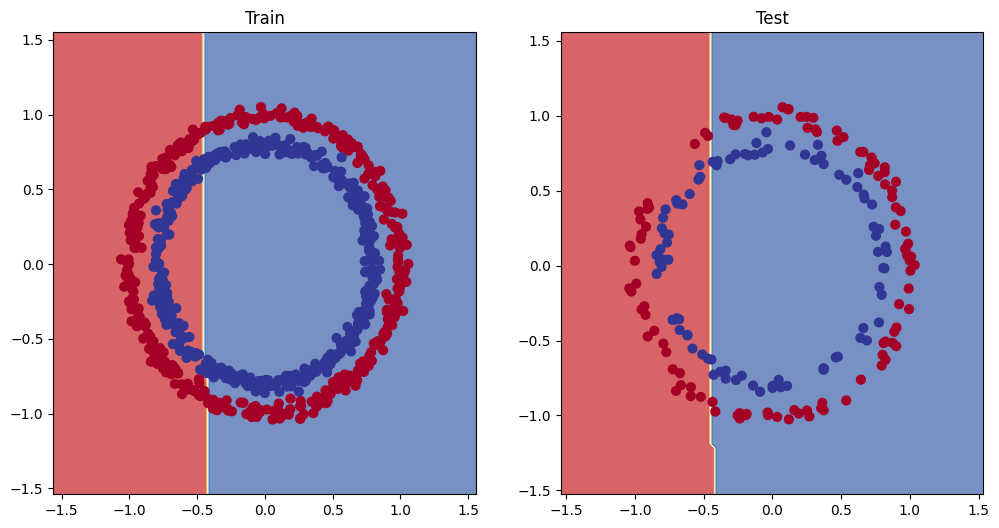
We know that by simply drawing a linear line through this dataset will not give optimal separation. This means that in case of a balanced dataset, the model will often stop improving around the 50% accuracy mark. This is where the loss function will be the lowest. If it moves towards solely predicting a one single class, it is pulled back by the other data points that do not line up with that class. On the other hand if one of the two groups is under-represented, the punishment to the loss function does not outweigh the gain made by the increase in prediction on one class. This means the model might reach higher levels of accuracy. But when honestly examining the model using the F1 score instead of the accuracy, you will see that it doesn’t model the data well.

We will talk more about metrics such as F1 score in a later session.

Simply put, we need to adjust our model to be able to fit the data.

↪️ Activation Functions

To allow our model to properly fit such data, we need to escape linearity. This is done by so-called activation functions. Borrowing their name from the biFological neurons and how they decide to ‘activate’ or not, activation functions serve a similar purpose. A function is applied on the output of a linear neuron. This function thus changes the outputs of the layers. This is more easily demonstrated in a visualization.

Figure 5: Various activation functions applied to a linear line

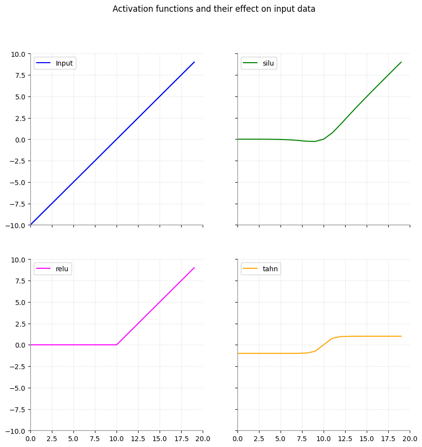
Image originally from my MA thesis.

In the image you can see how the top left linear line changes when applying activation functions on these. This image only shows three common ones, namely:

• nn.SiLU()
• nn.ReLU()
• nn.Tahn()

There are a many more that you can find in the Non-linear activation functions documentation. But some other common ones you will often encounter are nn.GELU() and nn.LeakyReLU().

You can see that their effect on a linear line differs but in essence all allow the line to ‘curve’, introducing a factor of non-linearity. With these layers the model will be able to fit to non-linear data too.

🏗️ Model Construction - Non-linear model

Encoding these layers within our model is relatively simple.

# 1. Construct a model class that subclasses nn.Module
class NL_ModelV1(nn.Module):
    def __init__(self):
        super().__init__()
        self.network = nn.Sequential(
            nn.Linear(in_features=2, out_features=10), # takes in 2 features (X), produces 10 features
            nn.ReLU(), # ReLU activation added
            nn.Linear(in_features=10, out_features=10), # takes in 10 features, produces 10 feature
            nn.ReLU(), # ReLU activation added
            nn.Linear(in_features=10, out_features=1)
            )

    # Define a forward method containing the forward pass computation
    def forward(self, x):
        # Return the output of layer_2, a single feature, the same shape as y
        return self.network(x)

We can ‘pad’ the nn.linear() neurons in nn.ReLU() which reflects itself inside the network as all these neurons receiving that as an added activation function. This is also the reason we don’t start of with a nn.ReLU(), it holds a function and is not a layer of neuron in itself. Also take not that this means that our activations functions do not require any parameters to be passed to them. They always operate on the output of the neurons when placed in a network.

After repeating the training process, we then see the following decision boundaries, keeping all the other hyperparameters the same.

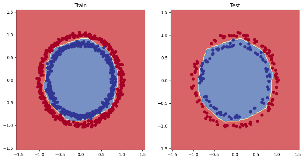
Figure 6: Model decision boundaries with nn.ReLU() after training

As you can see the model is able to bend its decision boundaries around the two groups and effectively separate the two classes!

🏆 Challenge

We have now fitted a model on the make_circles() with little limitations. In the real world you would not always have such freedom. The cost of GPU computing, time-limitations etc. all limit how large your model can be and for how long you can train it. In this challenge we try to mimic this a little with a constraint on the number of epochs.

Your goal is to create a model that fits the following data:

# Make 1000 samples
n_samples = 1000

# Create circles
X, y = make_moons(n_samples,
                    noise=0.15, # a little bit of noise to the dots
                    random_state=448) # keep random state so we get the same values

Which generates this:

Figure 7: Moons Data

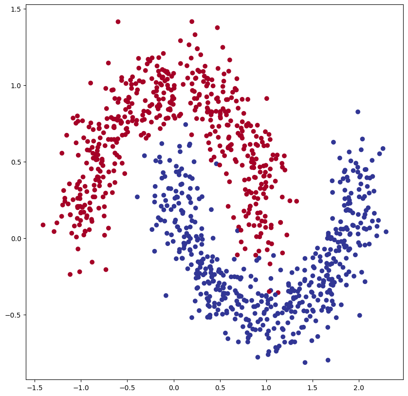
Your goal is to train a model with the highest accuracy within 800 epochs. Try to play with upscaling and y downscaling, test out different activation functions or combine different ones per layer.

📅 Next Session

Working with Images