💽 Session 5
Transfer Learning
💽 Transfer Learning & Fine-tuning
So far we have built a few models by hand. This should have provided you an understanding of how model architectures are developed. Performance on some basics sets has been surprisingly good. But when one moves to their own interest, you will quickly find that developing an architecture and training it from scratch is time-consuming and performance is often poor.
You might wonder, does a model exist for my problem? In most humanities cases, you will find that there are no models specifically designed for your particular problem. But, there are a LOT of models that have proven themselves on other tasks.
We can copy the architecture of these models and also their weights, and use them for our own tasks.
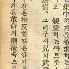
For example, we can take a computer vision model trained on ImageNet and use these weights to train it to e.g. identify the print shop of a colonial Korean magazine page scan.
Both research and practice support this.
Findings from a 2022 machine learning research paper recommend to use transfer learning whenever possible.
We also perform an in-depth analysis of the transfer learning setting for Vision Transformers. We conclude that across a wide range of datasets, even if the downstream data of interest appears to only be weakly related to the data used for pre-training, transfer learning remains the best available option. Our analysis also suggests that among similarly performing pre-trained models, for transfer learning a model with more training data should likely be preferred over one with more data augmentation.1
There are two versions of this. Transfer Learning and Fine-tuning
Transfer Learning
Transfer learning involves repurposing a pre-trained model for a new, different task by leveraging the model’s existing knowledge. This method offers several key advantages:
This has a few advantages:
- Efficiency: Your model can reach high performance faster than if you train from scratch.
- Less Data: You need less data to reach a high performing model
- Reduce Overfitting: Working with fewer data means more chance of overfitting, this is less of a risk with transfer learning.
- Resource saving: Utilizing pre-trained models conserves computational resources.
In the transfer learning approach, the typical process involves freezing the pre-trained model’s layers to retain their learned weights, with minimal adjustments made, if any. This step ensures that the generalized knowledge acquired from the original training is preserved. The main focus then shifts to adapting the models’ classifier to a new task, while the core of the model remains unchanged and frozen.
Fine-tuning
Fine-tuning refers to a more involved adaptation of a pre-trained model to a new task, where, in contrast to transfer learning, the emphasis is on adjusting the entire model. Key distinctions include:
- Complete Model Adjustment: Unlike transfer learning, where layers are frozen to retain their learned behaviors, fine-tuning involves unfreezing the entire model. This allows for comprehensive retraining and adjustment of the model’s weights to the specifics of the new task.
- In-depth Learning: By retraining the whole model, fine-tuning facilitates deeper learning adjustments that are more finely attuned to the new task, potentially leading to superior performance.
- Flexibility: This approach offers the flexibility to significantly modify the model’s learned patterns, making it particularly effective when the new task differs more substantially from the tasks the model was originally trained on.
A downside here is that it fine-tuning requires more computational resources.
Where to find models?
| Location | What’s there? | Link(s) |
|---|---|---|
| PyTorch domain libraries | Each of the PyTorch domain libraries (torchvision, torchtext) come with pretrained models of some form. The models there work right within PyTorch. | torchvision.models, torchtext.models, torchaudio.models, torchrec.models |
| HuggingFace Hub | A series of pretrained models on many different domains (vision, text, audio and more) from organizations around the world. There’s plenty of different datasets too. Lately, HF has been the hub for any activity related to open-source LLMs | https://huggingface.co/models, https://huggingface.co/datasets |
| timm (PyTorch Image Models) library | Almost all of the latest and greatest computer vision models in PyTorch code as well as plenty of other helpful computer vision features. | https://github.com/rwightman/pytorch-image-models |
| Paperswithcode | A collection of the latest state-of-the-art machine learning papers with code implementations attached. You can also find benchmarks here of model performance on different tasks. | https://paperswithcode.com/ |
Today we will focus on using the built-in PyTorch models.
🗂️ Data folders
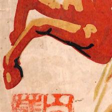
The data we will be working with is the data I discussed. Cutouts of uninformative training samples in my print shop research.
Please download it here.2 This will contain a folder with 2 folders. Good/Bad images. Unzip it and upload it to the Google collab folder your notebook resides in.
2 This link has been removed as it was only available during the workshop session.


To make use of such a folder we can use ImageFolder from torch.utils.data
from torchvision import datasets
from torch.utils.data import random_split
import torch

# Load the complete dataset
complete_data = datasets.ImageFolder(root='bad_imgs_dataset',
                                     transform=data_transform)

class_names = complete_data.classes

# Define the sizes for your training and test sets
total_size = len(complete_data)
train_size = int(0.8 * total_size)  # e.g., 80% of the dataset
test_size = total_size - train_size  # the rest goes into the test set

# Split the dataset
train_data, test_data = random_split(complete_data, [train_size, test_size])

print(f"Train data size: {len(train_data)}\nTest data size: {len(test_data)}")
This will then load the images, which we can use in Dataloaders again.
from torch.utils.data import DataLoader


# Define batch size
BATCH_SIZE = 32  # You can adjust this size depending on your memory capacity

# Create DataLoader for training data
train_loader = DataLoader(train_data, batch_size=BATCH_SIZE, shuffle=True)

# Create DataLoader for test data
test_loader = DataLoader(test_data, batch_size=BATCH_SIZE, shuffle=False)
💽 Loading a pre-trained model
In this example, we will load the Efficientnet B0 model. This model offers a good balance between number of parameters and performance.
Find it in the table here and specifically here
Before we can load the model, we will need to load its transforms. All pre-trained models have conducted some operation on the images they were trained on. Often this involves a crop and resizing of the input images, but when using the model pre-trained we also need to take into account the images that it has learned on. There is a mean and standard deviation associated with these that we also apply to our images.
We can load this manually by inspecting the model page, or automatically by letting PyTorch handle this. In this case, we will let PyTorch handle it.
We first load the weights, that have linked to them, the transforms.
# Get a set of pretrained model weights
weights = torchvision.models.EfficientNet_B0_Weights.DEFAULT # .DEFAULT = best available weights from pre-training on ImageNet
weights

# Get the transforms used to create our pre-trained weights
auto_transforms = weights.transforms()
auto_transforms

# returns:
ImageClassification(
    crop_size=[224]
    resize_size=[256]
    mean=[0.485, 0.456, 0.406]
    std=[0.229, 0.224, 0.225]
    interpolation=InterpolationMode.BICUBIC
)
Why would we use manual transforms? If we want to add irregularities to our images so the model can learn better. We won’t go into this now, but Albumations has a great page explaining the concept.
Now, we can load this model simply with the following line:
model = torchvision.models.efficientnet_b0(weights=weights).to(device)But this model will not work for use yet. We need to adjust the final layer, that one is now stuck on the ImageNet settings.
we can do this by first inspecting the last layer manually (printing out the model) and scrolling to the end. In efficientnet, the last layer is referred to as the classifer but in other models you will find it named differently, so we can not automate this easily.
model.classifier

# returns
  (classifier): Sequential(
    (0): Dropout(p=0.2, inplace=True)
    (1): Linear(in_features=1280, out_features=1000, bias=True)
  )
We then copy the classifer into a nn.Sequential but adjust the out_features. we overwrite the previous classifier.
model.classifier = nn.Sequential(
    nn.Dropout(p=0.2, inplace=True),
    nn.Linear(in_features=1280, out_features=len(class_names))
)
Right now we have a network ready for fine-tuning. But this is computationally more intensive. Let’s see if we can get good performance with freezing the rest of the model.
# loop through named layers
for name, param in model.named_parameters():
  # check if 'classifier' is in not in name as we don't want to disable that
  if 'classifier' not in name:
    param.requires_grad = False
  print(name, param.requires_grad)
This ensures that all the layers are turned ‘off’ - frozen as they do not keep track of gradients. Except of course, if it is the classifier.
Then we can proceed to training as before and see the results!
